| Log In | Not a Member? |
Support
|
|
|
Throughput and LatencySome programmers write functions that do a small amount of work on a data atom and return a result. They optimize the function to do its task and return as quickly as possible. This is frequently described as the low-latency approach to optimization, because it seeks to reduce the function latency -- the time between when a function is called and when it returns. Low-Latency functions are simple and easy to use. Data is traditionally passed by value and functions are typically small. On the other hand, when the overall goal is to complete an operation on your entire data set as quickly as possible, rather than just a small fragment of it, pursue a high-throughput design. High throughput designs are those that focus on moving as much data through the calculation as possible in the shortest amount of time. In order to achieve that, any part of the calculation that doesn't need to be repeated for each new piece of data is moved out of the inner loop. Just the essential core operations are repeated for each data. These functions can be complex and are most effective when operating over large data sets. In C, they are usually passed data by reference. They also typically have a higher up front overhead. Calculation Time = Overhead Time + Data Count / Throughput Overhead in AltiVecOverhead associated from AltiVec arises from a few different factors. These include the cost of saving and restoring vector registers, organizing data within register, and loading / assembling constants for use in your function.Register Save and RestoreSetting up a stack frame for a function that uses AltiVec is more expensive than for other types of functions. This is true for two reasons. To begin with, the vector register file holds a lot of data. The 32 AltiVec registers together hold 512 bytes of data. Saving their contents and restoring them involves more of the caches, meaning that more other important data may be flushed out. In addition, the cost of other tasks that involve saving or restoring vector registers such as exception handling or thread context switching can also be larger due to the need to save and restore registers. So that the processor doesn't have to save and restore every vector register every time an exception is thrown or there is a thread context switch, the processor maintains a special purpose register called Data OrganizationThe fact that a vector register can hold many data at a time means that the developer must address the new problem of how data is organized within the vector register. If data is stored in memory in some format that is not especially suitable for the vector unit, there may be some up front cost to reorganizing the data for efficient calculation in register. One example of this was given in the Data Handling section. Another example might be unaligned vector loads. These require that you load N+1 aligned vectors and do N permutes to move N unaligned vectors in to register. Clearly if you only load one unaligned vector in your function as part of a low-latency design, you will be paying an extra 100% load overhead, but if you load 10 vectors then the added load will only constitute a 10% extra overhead, and 100 vectors will only have 1% overhead. ConstantsFinally, constants are not as easy to generate in the vector units as they are in the scalar integer units. Getting them into register may involve a load from memory or a series of operations to synthesize the constant in register. Vector constants also take up more room in the caches. Overhead SummaryAltiVec functions can have substantial setup cost compared to their scalar counterparts. It is important to minimize the fractional overhead contribution to the cost of the calculation as a whole, in order to avoid having the overhead become the dominant time component in your function. The best strategy is to try to pay the setup cost once and then amortize it over as much data as possible. Very small AltiVec functions with non-trivial setup costs can be slower than their scalar counterparts, so these are best avoided. Low latency functions are usually only a large performance win if they are inlined. Throughput -- Pipelines, Parallelism and Superscalar executionThe other half of the speed equation is the throughput of the core calculation. The vector unit has a very large capacity to do work. It can begin executing two or three vector instructions in each cycle, and up to eleven or twelve instructions may be in the execution units concurrently, involving up to 32 vectors. This means quite a lot of data in flight at any given moment. How is it that all this data can be in motion at once? A common problem in processor design is that some operations take quite a long time. If you waited for one operation to complete before starting the next one on the same unit, it would be quite slow. A solution to this problem is to break down the calculation into many shorter steps, similar to an automobile assembly line. As the clock advances, intermediate calculations are advanced down the assembly line from one pipeline stage to the next until a finished calculation emerges at the end of the pipe. As a calculation moves from stage 1 to stage 2, another instruction can move in behind it and occupy stage 1. With the next tick of the clock, the first instruction moves to stage 3, the second to stage 2 and a third instruction can begin execution in stage 1 and so forth. Were this process to go on long enough, we would achieve a throughput of one instruction completed per cycle, and the pipelines would be full of data undergoing calculation:  The AltiVec unit, load store unit and the scalar floating point unit are pipelined. The following table details the number of stages in the vector execution unit pipelines of the different G4 generations:
In addition, the AltiVec unit is capable of superscalar execution. This means that the processor can start executing instructions on multiple units in the same cycle. The PowerPC 7400 and 7410 can dispatch two instructions per cycle to different execution units. Up to two of these may be vector units. However, only the permute unit is capable of receiving simultaneous dispatch with any of the other three vector units on the 7400 and 7410. If you need to dispatch a complex and a simple vector integer instruction, then they must happen on separate cycles on those processors. The PowerPC 7450 and 7455 can dispatch (send) up to three instructions per cycle. These must all go to different execution units, any two of which can be vector units. The third may be anything else, including a vector load, store or vec_lvsl / vec_lvsr. It should be clear now how 11-12 instructions can come to be executing concurrently. If we saturate the VFPU, VCIU and the load/store unit (which has a pipeline length of 3), we can have 11 or 12 instructions in flight at once. As each instruction can involve more than one vector, this could in principle involve up to 39 vectors in motion in a given cycle. In actuality, we only have 32 registers and it is pretty rare to use both the VFPU and VCIU at the same time, so this won't happen. A more likely scenario might be a code segment that keeps the VFPU, VPERM and LSU units busy all at the same time on the PPC 7450/7455. This is fairly typical of what you would see with basic linear algebra functions that deal with unaligned vectors. Similarly, you could have the VCIU, VPERM and LSU all busy in typical functions involving unaligned pixel buffers. Functions of this type could involve up to 27 vectors in flight at any given cycle. (This is derived from 4 vec_madd, 2 vec_perm, and 3 vec_ld executing concurrently.) That is a few vectors short of half a kilobyte! If you write low latency functions that only consume a vector or two of data before returning, you won't be making the most of the vector unit. The G5 can dispatch 4 instructions per cycle plus one branch instruction. Its dispatch limits are similar to the 7400, however. Only one permute and one VALU instruction may be dispatched per cycle. Up to two vector loads or one vector load and one vector store can also be dispatched that cycle. Latencies are one cycle longer to move data back and forth between the permute unit and the VALU. Loading data to the permute unit takes four cycles. To the VALU takes five. The key to achieving maximum sustained performance in the vector unit is to keep the execution units busy all the time. For our initial discussion about how to do that, we will provide some examples using the scalar FPU, because it makes for simpler examples. There is only one FPU instead of the four vector units, and scalar floating point code is compact and easily understood. However, as we will show at the end, exactly the same principles apply to the vector unit. We shall warn you ahead of time that the simple function that we will choose has some serious performance problems, as many simple functions do. It will be a long and difficult road to bring its real world performance up to something that comes close to saturating the FPU. Hopefully the trip will prove educational, and you will have a better idea what sorts of things help and harm processor performance.
Data Dependency StallsThe trouble with pipelines and superscalar execution is that they don't do you any good if you don't give the execution units enough work to keep them busy. Let's take a simple scalar function as an example:
Ignoring for the moment the task of loading and storing data and any work required to set up and take down the function's stack frame, this compiles to two
The problem with this is that each instruction depends on the result from the instruction before it, so one instruction can not start executing until the one before it moves all the way through the pipeline. On PowerPC 7450 and 7455, this means 5 cycles for each instruction for a total of 15 cycles to finish this three instruction sequence. During that time, four out of five of the pipeline stages are empty at all times, meaning that the FPU is only doing about 20% of the work that it is capable of doing in that time. Here we depict the 7450/7455's five stage FPU pipeline, and the progress of the instructions as time progresses (cycles 1 - 15).
Now, suppose instead we had written this function to do five dot products simultaneously:
Again, ignoring the problem of loads, stores and stack frames, we now have five
Given our hypothetical perfect pipeline, in 19 cycles, you would be able to complete five dot products! Since 15 is not a lot different from 19, the developer might choose to write his dot product function to always do five at a time, even if he didn't always have five dot products to do. If all you have is two dot products to do, you will be nearly twice as fast using that function than you would if you twice called a dot product function that only does one dot product. It would also be a constant reminder that you could be doing more work in parallel, every time you use it. More than One PipelineWhat happens when there is more than one pipeline? There are two different kinds of scenarios here that need to be discussed. Parallel PipesWhen there are two pipelines that do pretty much the same thing — e.g. the G5's dual floating point units or dual load/store units — then the two pipes operate in parallel, as long as there is enough data to keep them full. Looking at the G5's pair of FPUs, each has a pipeline length of 6. As long as there are 12 (6+6) independent operations that are able to execute, the pipelines will be full and the FPUs executing to capacity. If the series of sequential operations are dependent on one another, such that the result of one is required to begin calculation on the next, then the FPUs will be largely under utilized and one might not get used at all. For simplicity's sake, you can think of the dual FPUs as a single double clocked 12 stage FPU. This ignores some important dispatch limitations, but it is a good start and will help you understand the degree of parallelism required in your code. Most of the examples below focus on the 7450's 5 cycle FPU pipe. To do similar things on a G5, we would want to unroll the loops by 12 instead of 5. Happily unrolling by 12 will work fine on a G4 or G3 too. Extra parallelism rarely hurts. Serial Pipeline LimitationsPipelines can also be organized by code to operate serially with one another. For example if you do a load, add then store, then you have linked the LSU, FPU and LSU again in series to get the job done. This can change the throughput characteristics of the entire system, because the FPU isn't the only potential bottleneck anymore. To continue with our example, we must ask whether the claim is realistic that we can do 5 dot products in 19 cycles as claimed in our theoretical discussion above? Can we really get five dot products done in scarcely more time it takes to do one? Yes, and no. We can stuff the pipelines like that and get a lot more done in the FPU in roughly the same amount of time. However, we can only do that in practice if all the data is in register, ready to enter the pipeline at the moment it is needed. Clearly we have ignored in the discussion so far any load or store instructions needed to get the data in and out of register, as well as any stack setup costs. What really happens with these two functions when the full picture is taken into account? Below are shown actual execution times for these functions on a PowerPC 7450, when called in a tight loop:
What was wrong with our original approach? As it turns out, for every call to
To find out what really happened, we examine the code the compiler produced for
The first thing we find out is that both compilers just replicated the
The new code is faster (15%) and compiled as we intended but it is still not the huge speedup that we were looking for. (Recall that based on a perfect pipeline model, we were hoping for nearly a factor of five boost in throughput.) So, that is clearly not the complete story. The reader will note that our little optimization was still just a blind guess. We still haven't run the one clear experiment to find out why the two code samples do not perform significantly differently from each other! To find out what really happens, go to the trace. Sim_G4 will show us how exactly this code executes on a PowerPC 7400 or 7410. (Remember that the FPU pipeline is only three stages on those processors.) Here we see the first two dot products from DotFive():
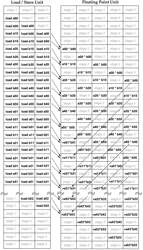
In this single trace, we find the complete story. So far as the instruction order is concerned, the first ten instructions are the first dot product. The second ten are the second dot product. The third ten instructions, if they were shown, would be the third dot product, and so forth. When talking about the order of appearance of instructions, the dot products don't intermingle. This does not mean however that the first dot product has to finish before the second one can start, even though they reuse the same registers. You can clearly see that they do in fact overlap as they execute: The first load from the second dot product (instruction 11 highlighted in red) was able to begin execution (regions containing 'E' or 'F') before the first dot product even started its second Multiply-Add Fused (MAF, instruction 9). In addition, though instructions 9, 10 and 12, (the last MAF and store from the first dot product, and the second load from the second dot product, blue) all use F0, they were able to execute all at nearly the same time, completing only one cycle apart. Thus, so far as the timing of instruction execution is concerned, there is a very high degree of overlap between the dot products, meaning that the LSU is a lot more full than the earlier simple models would imply. This is not to say that LSU usage is 100%. There is a two cycle "stall" between instruction 7 and 10 during which we begin executing no instructions in the LSU. This happens again after instructions 15 and 17. The reason our optimizations are not having a larger effect is that the original unoptimized code was executing a lot more efficiently than we originally posited based on the simple pipeline models presented earlier. Were these models wrong? No, not so far as they go. However, they did not take into account the interaction between multiple dot products called in series. Significantly, it is now clear that even with single dot products dispatched one after the other, the primary factor determining speed is not FPU usage. It is LSU throughput. When we reorganize the usage of the FPU so that we don't see stalls there, we force fewer LSU pipeline stalls. This is why the
You can see below why the DotFive2():
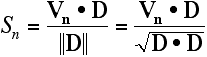
Write Non-trivial FunctionsIt isn't really that satisfying to leave our function limited by the performance of LSU. It is hard to get multiple GigaFLOP performance if you leave the FPU largely idle. What can we do to fix that problem? Unfortunately, there is not much we can do to change the fact that we have to load two data for every FPU calculation that we do in the DotProduct() function. That is just what dot products do. Therefore, all we can do is change the function to do some other calculation that does more work in the FPU per data loaded. It is often not hard to figure out what to do. Look at the caller. Find out what it is using the dot product for and merge that operation into the function, either directly or rely on the compiler to inline it for you. A dot product is fundamentally too simple to function efficiently -- it doesn't process enough data to keep the processor busy. A larger, more complex function can, however. This is a consistent trend that you will likely find in your code. Small simple functions are often the worst performers. We already described a situation where load throughput issues were causing performance problems in the Memory Performance section (that time due to limited throughput from loads that miss the caches). This is another. The solution to both is the same. Write less trivial functions so that you have enough work to do to fill the spare cycles. What we will seek to do is find ways to add more FPU instructions into the function without significantly worsening the load on the LSU. Because our dot product FPU pipeline is running less than half full, we hope that we will be able to squeeze much of the additional work into the available pipeline holes, thereby getting some or all of the work for free! Because we are doing the additional work now when it is free rather than later when we have to pay for it, we hope to see a net performance win in the application. Another way one might look at this is that we removed some load/store overhead. However this interpretation understates the gains we make using this sort of optimization. Because the LSU is the bottleneck, by removing these loads and stores, we not only avoid the LSU overhead, but also remove the downstream inefficiencies caused by the bottleneck. Thus, the net performance win is much more than the time cost recovered by removing the extra instructions in the LSU alone. Our Example Continues... Let us suppose that the reason we wanted to use the dot product was to calculate a Doppler effect for 3D audio for a game. To calculate the Doppler effect, we need to know how fast two objects are approaching each other. We want to find the speed S along the vector (D) between the listener and sound source. If the listener is at the origin and is not moving, this is calculated from the velocity (Vn) of the noise and the distance (D) as follows:
In a real program, we probably could have gone on to use that result to further calculate audio pitch deltas for each sound using the speed S along the D vector and perhaps audio gain settings, but this unnecessarily complicates the example. We have enough material to look at already. This problem is somewhat close to the problem of vector normalization that we described in the Data Handling section. Since we are still working in the scalar domain, and we are talking about filling pipelines, the routine we will present here will use all of the same ideas for the faster scalar vector normalization routine proposed there but not implemented. Specifically, division does not pipeline in the FPU. Also the sqrt() C Std library routine will break up our pipelines and in this particular case, sqrt() is unnecessarily precise -- we only need about 8 bits of precision to satisfy the Sound Manager volume functions. So that we can show full pipeline use through the entire function, we will use the Since the sound manager volume is quantized to 256 volume levels (provided we avoid Spinal Tap volumes) the full 23 bits of single precision accuracy are not strictly necessary, and so we will only go through one round of Newton-Raphson, providing about 10 bits of accuracy. We will rely on the compiler to properly schedule the instructions to fill as many pipeline holes as it can. We also rely on it to throw away some of the registers we declared, because we really don't need them all the whole time. This saves some stack overhead for saving and later restoring them at the beginning and end of the function:
The vector version of this function uses vec_rsqrte() in place of frsqrte, which provides 12 bits of accuracy. That is more than enough for our purposes, so we don't need to bother with Newton-Raphson in the vector case. Scalar ResultsHow did we do? Its a little difficult to run a side by side comparison between the scalar code and some other imaginary preexisting code in a non-existent game. However, we can verify that we did a better job of filling the FPU pipelines by returning again to the Sim_G4 trace. Because we show the vector code for this next, we can guess that the 7400, with SimG4 models, will never actually see this particular bit of scalar code. However for single precision floating point, the 7400 FPU is substantially like the G3, so it is a reasonable model to use. Here is a SimG4 vertical scroll pipe trace for the core function loop in execution:
In the above table, pipeline holes in the FPU appear as lines in the left column that are blank. The comments column names the various stalls we encountered along the way. Overall, we have done very well -- better than it might appear at first glance. The following section details each of the stalls that we see. Common Stalls You Will See in SimG4 Traces: The first comment we see "Maximum Allowed Dispatched" The PPC 7400 can only dispatch two instructions per cycle to all of the execution units in total. It can also only retire two per cycle. The PowerPC 7450/7455 can do three for both. When you see "Maximum Allowed Dispatched" you know that the processor is operating at maximum efficiency. This is not a stall. The Another thing you have to acquire before an instruction can enter execution is a rename register to help manage the process of writing your results to register and to help forward the data to other instructions that might need it immediately. The PowerPC 7400/7410 have 6 integer rename registers, 6 vector rename registers and 6 floating point rename registers. Since we can have 8 instructions in flight in the ICQ, it is possible that if nearly all of these write to any one register file that we will run out of rename registers for that register file. If your code strictly uses the FPU, this can't happen because the FPU pipelines are not long enough to saturate the rename registers. However towards the beginning of the function, we have both the FPU and the load store unit writing to the FP register file, so we do in fact run out of rename registers. This is where we see " Finally we see a number of instructions labelled One other optimization note: the compiler has added some
Scalar Performance DiscussionOur new function takes a standard dot product (D dot V) and appends a lot more work onto it, by adding a vector normalization, division and a second dot product using the same small set of data. What kinds of performance advantages did this buy us in the end? The instructions corresponding to what would be issued for a dot product function that does three dot products are shaded in blue the Sim_G4 results above. Nine of the 38 FPU instructions are from the original. The other 29 are new. Our changes introduced no new load/store instructions. We simply do more with the data while it is in register. As a result, a routine that was load/store bound is now primarily FPU bound again, which means our calculation throughput is approaching 1 FPU instruction per cycle. One can see this effect by comparing the percent utilization of the FPU for on optimized high throughput
We can also see this in terms of raw execution times. The function
The timings and the SimG4 trace above both suggest that by increasing the complexity of the calculation by a factor of four, we were able to saturate the FPU, saving quite a bit of time. Actual execution times only went up by a factor of two. Recall that this new function actually does two dot products. Our benchmarks show that calling Vector ResultsWe also present a similar trace for the vectorized version of the code. Compared to the scalar implementation, we save some time because we don't have to do a Newton-Raphson optimization step, but we have to surrender some time dealing with the interleaved float[3] data format, a format highly inconvenient for the vector unit.
The first vector version, vector 1, takes the same interleaved {x, y, z} data format that the scalar code used. The second vector version, vector 2, uses vector-friendly planar data format instead, which requires no on the fly internal format conversions before the data can be processed. This second variety is for those that are curious what these interleaved formats sometimes cost. In this case, 27% of our time goes to dealing with swizzling, and we can expect a 36% performance increase if we switch to planar data layouts. The four-fold parallelism in the vector unit lets us achieve throughputs of 3.3- to 4.2-fold higher than what we were able to get in the scalar units. Earlier we promised to show that the same processor features that lead to enhanced scalar performance are also at work in the vector unit. As a result, we now ask, how much better is this than the vectorized version of DotProduct() written using a low-latency design?
Here is the performance comparison between various flavors of the
What?! The low latency vector routine is slower? Yes, it is. Perhaps you might think we handicapped it by forcing the routine to return a float. Lets fix that:
Here is the performance comparison between various flavors of the DotProduct function again.
Clearly that wasn't the whole problem! Just to drive the point home, this is the speed difference between
Why is the low latency vector dot product itself 3.7 times slower than Vector Performance DiscussionThe problem with tiny low-latency vector functions is just as we described above for scalar functions, except worse because vector overhead is higher. We spend so much time dealing with overhead (setting up vrsave and coping with data layouts) that the overhead itself becomes the dominant time consumer in the function. If we look at it, we find that
To begin with, we see above that we have to spend a cycle or two generating the zero constant, and (unseen) we also some more time setting up the
Next, the multiplication operation is only 3/4 efficient, because there is a do-nothing element in the fourth position on each vector. We waste a little time there. Also, because the VFPU pipeline is 4 stages long, we take a three cycle stall while we wait for vec_madd to complete before the next instruction can start.
We now have to sum across the vector. The problem is that because we are using a non-uniform vector, the Y and Z components are in the wrong place to add to the X component. Thus, we have to do two left rotates to fix the problem. In addition, because this routine is again data starved, we incur a total of six more cycles worth of stalls after the adds, before we can return the data. Also, the two adds are doing redundant work -- there is less and less parallelism in register as this stage nears completion.
Finally, the computer also has to restore the vrsave special purpose register. The good news is that the function does complete from start to finish about as quickly as one could imagine doing a single dot product in the vector unit. However, it seems that in the end, optimizing for latency alone costs us dearly for overall performance. We can make a somewhat boastful claim of a factor of 33 performance improvement between the low latency vector implementation and the high-throughput one. It should be clear that for proper performance of the vector unit, it is very important to make sure you give it enough work to keep it busy! More data will help fill the pipelines, and more data beyond that will help reduce the fractional cost of the function overhead. Compilers and InliningThe skeptical reader may have realized that much of the work we show here may normally be expected to be done by the compiler when it inlines small utility functions into larger routines. Much of what we have done above is exactly that. Unfortunately, compilers do not always inline things -- one did, one didn't when preparing these examples -- and even when they do, they are sometimes unclever about how they do it. A compiler could in principle take a low latency function found in a loop, inline it, unroll the loop to cover the pipeline lengths and schedule everything to avoid pipeline bubbles and move one-time calculations out of the loop, thereby converting a low latency C function into high throughput assembly automatically for you. For whatever reason, this didn't happen in the examples presented here, so the improvements from inlining were modest. That is why it makes sense to verify the compiler is doing what you expect with performance sensitive code. In addition, often you might need to merge code horizontally between two functions called one after the other that operate on the same buffer. Sometimes these code segments may come from parts of the application called at very different times. Few compilers yet implement features like loop fusion or the high level of analysis required to make code move large distances. Thus, with today's compilers the notion of high throughput vs. low latency design for your functions remains important for proper performance in both scalar code and AltiVec. SummaryThe PowerPC processor is capable of dispatching multiple instructions per cycle into many parallel execution units that have pipelines many cycles deep. To saturate this system requires much more data than is typically passed into small functions. In some cases, an AltiVec function is capable of operating on as much as half a kilobyte of data at any given time. Thus, low-latency designs often leave the processor data starved and performance suffers greatly. In order to overcome these problems, the high throughput design must seek to keep ALU pipelines full. In many cases, this may mean that the functions themselves must be redesigned to do non-trivial amounts of work and operate in concert with better temporal locality of data reference. The end result can be a many-fold rate acceleration in the operation of the function. This is true even of code that uses only the scalar units.
|


|
Get information on Apple products. Copyright © 2008 Apple Computer, Inc. |