|
Software Pipelining
Introduction
There is one last technique in the arsenal of the software optimizer that may be used to make most machines run at tip top speed. It can also lead to severe code bloat and may make for almost unreadable code, so should be considered the last refuge of the truly desperate. However, it’s performance characteristics are in many cases unmatched by any other approach, so we cover it here. It is called software pipelining, or sometimes loop staggering or loop inversion, because the inner loop does the operation in backwards order from the starting algorithm. It can be applied in varying amounts, resulting in varying levels of code bloat.
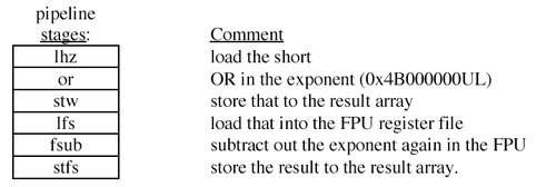
TheorySoftware pipelining at its core seeks to model a calculation as if it was actually implemented in hardware as a single instruction with a multistage pipeline. With each new virtual CPU cycle, a new piece of data is added to one end of the virtual pipeline and a completed result will be retired out of the other end. Why do that? Well some of the same factors that make this technique useful in hardware also lead to high performance in software. In particular, it leads to a high degree of parallelism, which works well with modern superscalar cores. In addition, in implementation it usually does a good job of hiding latencies for any particular step in the process. When done properly, an algorithm can be made to perform as if each of the instructions that make it up has a single cycle latency. You will likely be able to take advantage of maximum dispatch bandwidth available most cycles, so multiple things can be done concurrently. Even more fun, you can do multiple steps concurrently even if one step normally would depend on the result of the step before it before it can start. We will take as our working example the conversion of 16 bit integers to floating point values. On PowerPC, there is no direct conversion for ints to floats in hardware. Everything is done in software. The algorithm used here is a small modification on the algorithm presented in the IBM PowerPC Compiler Writers Guide, except that we use a float instead of a double for transferring data between the integer register file and the floating point register file. (There is no publicly exposed direct path.) Shown below are the six instructions that make up the operation in order, presented as stages in a hypothetical hardware execution unit that would do this operation:
Each of the stages is named after the PPC instruction that actually does that step.
Now, of course, no pipelined execution unit really functions to its fullest potential unless we keep it busy by pushing new data into it every cycle. Thus, in ideal operation, the actual execution of our virtual pipeline would look like this:
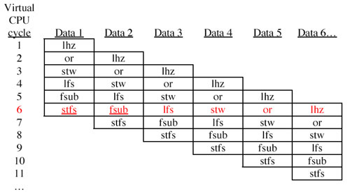
All of that is very nice, but as we don’t actually have a pipelined instruction in hardware, what good is it? Well, look what happens once we map this virtual pipeline to real instructions. To do that, we simply say that the code will be executed in the order shown in the diagram above -- left to right, top to bottom, in the same order as reading a book in English. This would be lhz, or, lhz, stw, or, lhz, lfs, stw, or, lhz, fsub, lfs, stw, or, lhz...
We will use virtual cycle 6 as an example (red) to see what happens once we get to the point when the pipeline is full of data. Notice that in this virtual CPU cycle, we have to do 6 different things. The six things are essentially our starting algorithm, except executed in reverse order. None of the data used by any of these instructions relies on the results from the other instructions in that row, so they can all be done in parallel, subject to the limitations of the parallelism of the machine. Happily, they use a lot of different execution units, so we may imagine that many of them are in fact executed in parallel – the PowerPC can dispatch and retire two or three instructions per cycle. For example, we might imagine that both the stfs and fsub (underlined) can enter execution in the same cycle because one is performed by the LSU and the other by the FPU.
In addition, though there is a ton of code here, register pressure is actually quite light because the registers are tied to the pipeline stages. When the virtual pipeline is full of data, every virtual CPU cycle uses every register that we declare. So we don’t have any data sitting stagnant in registers waiting for the right part of the loop to roll around.
Code like this is highly likely to saturate the capacity of the CPU for getting work done. This is promising!
Implementation
How does this look as C code? Because there are so many different things going on concurrently, it has the potential to look pretty ugly. However, with some use of the C preprocessor, we can make some sense of it. The basic loop structure looks like this:
void ConvertInt16ToFloat( uint16_t *in, float *out, uint32_t count )

									{
union

										{
uint32_t u;

										float f;

										}buffer;

										register float expF;

										register uint32_t expI;

										register uint32_t stage1_result, stage2_result;

										register float stage4_result, stage5_result;

										register uint32_t *stage3_target = (uint32_t*) out;

										register float *stage4_src = out;

										register float *stage6_target = out;

										register int i;
//Set up some constants we will need

										buffer.u = 0x4B000000UL;

										expF = buffer.f;

										expI = buffer.u;
i = 0;
if( count >= STAGE_COUNT - 1 )

										{

										//Some of the stages advance pointers in addition to

											//their stated operation.

											//STAGE_1 increments i in addition to loading in the uint16_t
STAGE_1;


											STAGE_2; STAGE_1;


											STAGE_3; STAGE_2; STAGE_1;


											STAGE_4; STAGE_3; STAGE_2; STAGE_1;


											STAGE_5; STAGE_4; STAGE_3; STAGE_2; STAGE_1;
while( i < count )

											{
|
STAGE_6; |
STAGE_5; |
STAGE_4; |
STAGE_3; |
STAGE_2; |
STAGE_1; |
}
|
|
STAGE_6; |
STAGE_5; |
STAGE_4; |
STAGE_3; |
STAGE_2; |
|
|
|
STAGE_6; |
STAGE_5; |
STAGE_4; |
STAGE_3; |
|
|
|
|
STAGE_6; |
STAGE_5; |
STAGE_4; |
|
|
|
|
|
STAGE_6; |
STAGE_5; |
|
|
|
|
|
|
STAGE_6; |
}
//Cleanup code for small arrays when count < STAGE_COUNT - 1

										while( i < count)

										{
STAGE_1;

											STAGE_2;

											STAGE_3;

											STAGE_4;

											STAGE_5;

											STAGE_6;
}

										}
All that is left to do now is define what the various stages in the software pipeline do. As a general rule, each of these should be a single PPC instruction. However, in certain cases you may need to also advance pointers or deal with loop counters. Those can be separate stages or just lump in the overhead to the formal pipeline stages. We have lots of integer units to do that work. The compiler will (we hope) find some nice place to squeeze in the extra work without causing trouble. The six STAGE_#’s we show here are the six stages in the virtual pipeline that we showed right at the beginning, written in C, with a bit of pointer arithmetic and loop overhead sprinkled in.
#define STAGE_1 stage1_result = (in++)[0]; i++ /* lhz */

											#define STAGE_2 stage2_result = stage1_result | expI /* or */

											#define STAGE_3 (stage3_target++)[0] = stage2_result /* stw */

											#define STAGE_4 stage4_result = (stage4_src++)[0] /* lfs */

											#define STAGE_5 stage5_result = stage4_result – expF /* fsub */

											#define STAGE_6 (stage6_target++)[0] = stage5_result /* stfs */

											#define STAGE_COUNT 6
You do need to be careful about data dependencies between stages. Data that flows through the pipe needs to move to a different storage spot each cycle to avoid having the data behind it overwrite it. Thus, destructive operations are likely to cause trouble. Example:
#define STAGE_1 a = (array++)[0];

											#define STAGE_2 a += b; /* destructive! */

											#define STAGE_3 (resultPtr++)[0] = a;
Here, the variable ‘a’ was already modified in STAGE_1. You shouldn’t modify it again in STAGE_2, or that result might be fed into STAGE_2 again in the next virtual cycle. When this is inverted inside the inner loop, it will lead to some curious results that you had probably not intended.
The key is to just make sure the data keeps moving each cycle. The following fixes the problem:
#define STAGE_1 a = (array++)[0];

											#define STAGE_2 c = a + b; /* non-destructive */

											#define STAGE_3 (resultPtr++)[0] = c;
Data that is not in register can afford to stay in place, but you need to update the pointers each cycle so that the next virtual cycles' work doesn't overwrite the work done by the current one.
Performance Impact
The performance impact of software pipelining can be many fold for short functions involving high latency instructions, such as this one. For other functions with lower latency operations it may be only a small win (30%), but is usually faster than any other approach.
For large algorithms involving many, many pipeline stages, the code may actually run more slowly because of its size – the code may displace much needed data in the caches. Software pipelining causes software to grow to be N2 instructions, where N is the number of instructions in the inner loop of the unoptimized function, so its use should be limited to simple operations. For N is greater than 20 or 30, you also run the risk of running out of registers.
This particular code organization style is often good when applied locally to functions that are executed frequently, but bad globally for code bloat reasons. As a result, it is generally not done automatically for you by the compiler which usually has no idea which functions are executed frequently and which are not, though some compilers will do it at aggressive optimization levels.
How does our example perform? You may find the complete source for this example. It times the standard int to float conversion from your compiler, a simple version using the algorithm presented here and finally the software pipelined version. The correctness of each is verified. It may be compiled with gcc as follows:
Times to convert 1024 uint16s to floats (microseconds, G4/800 powerbook):
|
Native compiler conversion
|
simple
|
software pipelined
|
|
44.6
|
54.8
|
22.1
|
This native compiler method is provided as a speed baseline. The “simple” code is our exact algorithm, written in the mundane way. Rescheduling it using software pipelining gives us almost a 2.5x improvement.
Note: In many cases, code that has been software pipelined is almost perfectly scheduled for speedy execution on the processor. Most compilers tend to move loads early in the loop and stores late to cover data dependencies between loads and later instructions that need the data. However, we already established all the operations in a particular virtual CPU cycle (i.e. within the inner loop) have no such dependencies within that cycle (loop iteration). Thus, moving loads and stores around usually turns out to be the wrong thing to do. (While usually a win for most code, our code organization is arguably highly unusual, so it presents something of a problem for us.) You may find examples of software pipelined code that actually runs faster with some parts of the compiler optimizer turned off. Be careful not to turn too much off, or else you may introduce a lot of gratuitous loads and stores.
Keep it Simple
Its not always necessary to completely invert the loop as shown above. Often you can get an acceptable performance improvement by keeping the number of virtual pipeline stages to two or three, with each stage doing a lot of work. This is a good strategy for dealing with code bloat, as the actual number of instructions is N x stage_count, not N2. This sort of approach can be helpful for larger functions.
The logical extreme in this direction would be to concatenate all the load instructions into one stage, and the rest of the calculation into the other stage. The loop structure then becomes:
LOAD_STAGE;

											while( --count )

											{
CALCULATION_STAGE; LOAD_STAGE;
This simple staggering will often give you a 20% speed improvement over an implementation that looks like this:
LOAD_STAGE;

												CALCULATION_STAGE;
…and requires no cleanup loop at the end for small arrays, where count is less than the number of stages -1. We choose load instructions because they often have high latencies. Code organized this way can do its loads concurrently with the work.
Table of Contents NextPreviousTop of Page NextPreviousTop of Page
|