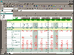
Helen Bradley looks at some of the options for naming cells on a worksheet to save you time and help eliminate errors in formulae, printing and moving around.

Figure 1c: If you name the cell containing the markup value, calling it Markup, you can refer to this name rather than the cell reference in formulae.
Most spreadsheet packages allow you to name a cell or a range of cells and to refer to this cell or cells by the name you have given them. Consider the example in Figure 1c: if you calculate the Markup for the first item, you'll enter =$B$4*B7 in cell C7 and then you'll copy this formula down the column. Alternately, if you name cell B4 'Markup' then the formula in C7 can be written as =Markup*B7.
To name a single cell or a range of
cells:
Step 1: Highlight the cell or cells to name.
Step 2: Select Insert, Name, Define. Excel will try and find a name
for your cell and will often get it right by taking a text entry from an adjacent cell.
Alter the proposed name in the Names In Workbook text box, if necessary, and click OK.
You can use any combination of characters for a name, but it must begin with a letter or
an underscore and you may not use a space or a hyphen. Names are not case sensitive and
the name 'Sales' is the same as the name 'SALES'.

Figure 2c: Using a combination of named ranges, macros and buttons on your sheet you can make it easy to print different areas of a sheet.
.
Names make formulae easier to understand. For example, the formula =C6*C7 means very little but if you were to name each cell and use the names in your formula then LoanAmount*InterestRate would make a lot more sense.
Names are easier to remember and use than are cell references. If you need a name in a formula you can 'look up' the names available using Insert, Name, Paste and select a name from the list. This menu option is available anytime you are building or editing a formula provided you have at least one named cell on your worksheet. Alternately, pressing F3 will bring up the Names list or you can click on the Names list on the toolbar, which you can see open in the top-left corner of Figure 2c.
You can redefine names and any formula using the name will automatically be recalculated to refer to the new range. So, if you have a lookup table named LookUpTable, and you add another two rows to the bottom of the table, you can redefine the name by selecting Insert, Name, Define and alter the range in the Refers To text box. Automatically all formulae in the worksheet that refer to the named range will now see the new, larger lookup table.
You should use range names to create databases, charts and print areas where you're likely to add or remove rows or columns within the area covered by the name. If you do this to within an area covered by a name, then that named range will expand or contract accordingly. You won't have to alter the database, chart or print area as a result of your changes.
When you've created a name on a worksheet, the name will not be used in any existing formulae unless you specifically apply it. To do this, select Insert, Name, Apply and select the names you want to replace ranges in any formulae in your worksheet. Leave the Ignore Relative/Absolute check box checked, leave Use Row and Column Names checked if you want to use references to intersecting cells (see below) and click OK. Now the named ranges will replace all cell references in your formulae.
You can use names to move quickly around your workbook. The F5 (GoTo) key or Control+G brings up a list of names from which you can select the name to move to and click OK..

Figure 3c: Once you have named a group of cells you can use these names in formulae and refer to cells at the intersection of two names.
If you have two areas of a sheet using names, you can create a button on the worksheet, to move from one area of the worksheet to another, or you can create buttons to print varying areas of a large worksheet. In Figure 2c each of the buttons allows a separate, named area of the worksheet to be printed. To create each of these buttons:
Step 1: Highlight and name each area of the worksheet that you want to print, leaving out the 'heading' columns A and B. In the budget worksheet the area C1:F22 has been named Quarter1, the area G1:J22 has been named Quarter2 etc.
Step 2: So that each area will print with the heading columns A and B, select File, Page Setup, select the Sheet tab and in the Print Titles area enter in the Columns to repeat at left: $A:$B and click OK.
Step 3: Record a macro which uses the GoTo command (F5) to go to the area to print, for example, Quarter1, then sets the print area using File, Print Area, Set Print Area and then prints using File, Print, Selection and which finally removes the print area using File, Set Print Area, Cancel Print Area.
If you prefer, type this macro in using Tools, Macro, Macros, key in the Macro Name as PrintQuarter1 and from the Macros In list box select This Workbook, select Create and type in this macro text:
Sub PrintQuarter1()
' Print Quarter1 of worksheet
Application.Goto Reference:="Quarter1"
'ActiveSheet.PageSetup.PrintArea = Selection
ActiveSheet.PageSetup.PrintArea = ActiveCell.CurrentRegion.Address
Selection.PrintOut Copies:=1
ActiveSheet.PageSetup.PrintArea = ""
ActiveCell.Offset(0, 1).Select
End Sub
Step 3: Create a macro for each print area. You can record one for each print area or copy and paste the macro text altering any reference to Quarter1 or to a specific print area.
Step 4: Before you can add a button to your worksheet you'll need the Button tool on your toolbar. To add this, select View, Toolbars, Customize and select the Commands tab. In the Categories list select Forms and from the Commands list drag the Button command up onto the toolbar and click Close to finish.
Step 5: To add a button to your sheet, click the Button tool and drag a button in position on your sheet. From the Assign Macro list select the macro to run when the button is pressed (PrintQuarter1) and click OK. Alter the text on the button by right-clicking on it and changing the text to Print Quarter 1.
Step 6: Repeat Step 5 for every button you need on your worksheet.
You can name a group of cells using their column and row headings like those in Figure 3c with one command and use the resulting names in your formulae. Select the range including the row and column headings and select Insert, Name, Create. From the dialogue box choose to Create Names In: Top row and Left column (where the names appear) and click OK.
You can now use the names to create the totals for the worksheet. For example, the formula in cell B8 will be =sum(Income) as the name Income will have been created to refer to the range B4:B7.
When you have intersecting ranges such as North referring to B4:D4 and Expenses referring to C4:C7 you can use 'intersecting names' which are the cells at the intersection of two named ranges. For example, if you key into a cell =North Expenses, the cell will contain 10,000 the contents of the cell at the intersection of the row range named North and the column range named Expenses. To refer to an intersecting name use the row name, followed by a space and then the column name.
BUDGET.XLS, PROFIT.XLS & NAMES.XLS
These can be found in the interact\names\ folder on the CD.
In addition to naming cells in the current workbook, you can also refer to named cells in another workbook. For example, =Profit.xls!YearTotal can be entered in the current workbook and will contain the value from the cell named YearTotal in the file Profit.xls. You can also refer to intersecting names, for example, =profit.xls!North profit.xls!Income will place the figure from the intersection of the named ranges North and Income in Profit.xls in the current worksheet.
Names work at the level of the workbook so a range name is available to any sheet in a workbook. Sometimes, however, you may want to use the same name for a cell on a number of worksheets, for example, you may have a workbook of worksheets recording share information and want to name a cell on each sheet MarketPrice. To do this you'll need to create a sheet level name which you can do by adding the name of the worksheet and an exclamation mark before the range name. So this cell on the sheet1 will be named sheet1!MarketPrice and if the worksheet is called BHP then the cell name will be BHP!MarketPrice.
When you're using the named range on the sheet where it is created then you don't have to prefix it with the sheet name and an exclamation mark. So to use the named cell Sheet1!MarketPrice in Sheet1 you only need refer to MarketPrice. To use that named cell on another worksheet you will need to prefix the name with the sheet name and the exclamation mark.
Top of page |
WEB: |What's New
| Net Guides | Web Workshop | Net Sites | About PC User |
|