Keep track of your debtors with this spreadsheet project by Helen Bradley.

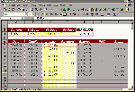
Figure 1b: This month's worksheet allows you to record details of outstanding invoices and analyse the age of these debts.
You will find examples of this in both Excel and Lotus 123 formats in the \INTERACT\DEBTORS folder on the the CD.
Although some of the formulae are specific to Excel, you can create the worksheet in Lotus too, and the box 'Lotus 97' explains the differences in the Lotus version.
Step 1: On a blank worksheet, add this data to the listed cells:
| Cell | Contents |
| A2 | 0 |
| B2 | 30 |
| C2 | 60 |
| D2 | 90 |
| E2 | 120 |
| A3 | Current |
| B3 | 30 Days |
| C3 | 60 Days |
| D3 | 90 Days |
| E3 | 120 Plus |
| A4 | =SUMIF($G$7:$G$200,"=Current",$C$7:$C$200) |
| B4 | =SUMIF($G$7:$G$200,"=30 Days",$C$7:$C$200) |
| C4 | =SUMIF($G$7:$G$200,"=60 Days",$C$7:$C$200) |
| D4 | =SUMIF($G$7:$G$200,"=90 Days",$C$7:$C$200) |
| E4 | =SUMIF($G$7:$G$200,"=120 Plus",$C$7:$C$200) |
| A6 | Date |
| B6 | Details |
| C6 | Invoice |
| D6 | Payment |
| E6 | Balance |
| F6 | Paid |
| G6 | Status |
| E7 | +C7-D7 |
| E8 | =IF(OR(C8>0,D8>0),+E7+C8-D8,"") |
| G7 | =IF(OR(F7="y",C7=0)," ",HLOOKUP(TODAY()-A7,$A$2:$E$3,2)) |

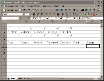
Figure 2b: Your worksheet should resemble this one when you have completed Step 2 of our instructions.
Step 3: Enter this data into the named cells to test the worksheet:
| Cell | Contents |
| A7 | 3/6/97 |
| B7 | #00105 |
| C7 | 200 |
| F7 | y |
| A8 | 3/7/97 |
| B8 | #00106 |
| C8 | 375.50 |
| A9 | 7/7/97 |
| B9 | #00105 |
| D9 | 200 |
| A10 | 3/8/97 |
| B10 | #00107 |
| C10 | 45 |
| A11 | 3/9/97 |
| B11 | #00108 |
| C11 | 275 |
| A12 | 3/10/97 |
| B12 | #00109 |
| C12 | 310 |

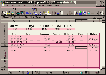
Figure 3b: This is the Invoice worksheet with the sample data in Lotus. The actual ages of each debt will depend on the current system date on you computer.
Step 4: You can add a warning to cell F4 which will check to see if you have entered an incorrect letter into any cell in column F or, worse still, a space. Key this formula into cell F4: =IF(COUNTIF(F7:F200,"<y")<>0,"Warning! Check Paid column",""). Format this cell in bold red type using Format, Cells and the Font tab. If everything is okay, you won't see anything in cell F4, however, if you enter a letter other than 'y' or a space in one of the cells in column F, you'll see the warning appear.
Step 5: Hide the numbers in row 2 by selecting the row number and then Format, Row, Hide. The numbers in this row are used only for reference by the HLOOKUP function and don't need to be visible.
Step 6: Format your worksheet attractively, making the data cells in columns C, D and E and in row 4 display numbers to two decimal places. Format all the way down to row 200 as there are formulae in all these cells. Remove your sample data and save the worksheet.
You can use this worksheet in one of two ways. You may choose to have one worksheet for each debtor, in which case you will need to prepare this worksheet and then copy it using Edit, Move or Copy sheet to create one worksheet for each of your debtors. In this case, renaming each worksheet to the name of the debtor is a good idea; do this by double-clicking on each worksheet tab and typing the debtor's name.
Alternately, you may choose to have one worksheet and to enter details of all your clients' invoices and payments into the one sheet. This way the sheet will give you a summary of all the money you are owed and a breakdown of the aging of these debts.
For each invoice include the date of the invoice, some identifying details and the Invoice amount. As each invoice is paid, record the payment details (date, details and payment) on a separate line and add a 'y' to the 'Paid' column opposite the invoice that the payment relates to.
When you have entered your invoice details, the last figure in the balance column will show you the current status of the debtor, or the total of your outstanding debtors, depending on how you are using the worksheet. The information at the top of the worksheet shows the relative ages of the debts.
The formulae in column E calculate the running balance by taking the total from the previous line and adding any Invoices and deducting any payments. The IF function merely tidies up the display by hiding the result if there's no value in the Invoice or Payment column.
The formulae in column G are more complex; they calculate the age of the debt by deducting the date of the invoice from your computer's system date. The number of days is passed to the HLOOKUP function which uses the table in the range A2:E3 and compares the number of days with the figures in row 2 to find the largest value that is less than that number of days. It then returns the corresponding value in row 3. So, if the debt is 0-29 days old, the value 'Current' is returned, if the debt is 30-59 days old the value '30 Days' is returned and so on. The IF part of this formula is there to neaten the display, it stops the calculations being made if the Invoice is paid or if there's no value in the Amount column.
The formulae in row 4 use a SUMIF function to add the values in the Invoice column only for certain criteria. The formula in cell A4 adds only those Invoice amounts for invoices that have 'Current' as the entry in column G, the formula in cell B4 adds only those Invoice amounts for invoices that have '30 Days' as the entry in column G etc. The syntax of the SUMIF function is =SUMIF(range to analyse,criteria,range to sum), so the formula in cell A4: A4 =SUMIF($G$7:$G$200,"=Current",$C$7:$C$200) translates as, sum the values in the range C7:C200 for those rows where the corresponding entry in column G is equal to 'Current'.
Finally, the formula in cell F4 uses the COUNTIF function which is similar to SUMIF. This counts the values in column F to see how many are less than 'y'. So if you've entered any alphabetical character (other than y and z) in column F or you've pressed the space bar, then the warning will display. This formula is very 'quick and dirty', it won't trap everything but it will catch the worst of your errors.
This worksheet can be easily created in Lotus 1-2-3. There are some differences in formulae, but the steps for creating it and the logic of how the worksheet functions are similar.
Lotus, however, doesn't have a SUMIF or COUNTIF function, so the DSUM and DCOUNT functions have been used instead. These functions require you to have a named area on your worksheet, so select the range A6:G200 and use Range, Name and name this area INVOICEDATA.
The other significant alteration is a rewrite of the formula in cell G7 to overcome Lotus' somewhat twisted logic that says that A=blank, B=blank but A<>B. Using the @ISSTRING function overcomes these difficulties.
| Cell | Contents |
| A4 | @DSUM($INVOICEDATA,"Invoice",Status="Current") |
| B4 | @DSUM($INVOICEDATA,"Invoice",Status="30 Days") |
| C4 | @DSUM($INVOICEDATA,"Invoice",Status="60 Days") |
| D4 | @DSUM($INVOICEDATA,"Invoice",Status="90 Days") |
| E4 | @DSUM($INVOICEDATA,"Invoice",Status="120 Plus") |
| F4 | @IF(@DCOUNT(INVOICEDATA,"Paid",Paid<>"y")>0, "Warning! Check Paid column","") |
| G7 | @IF((C7=0)#OR#(@ISSTRING(F7)#AND#F7="y"),"",@ HLOOKUP(@TODAY-A7,$A$2..$E$3,1)) |
| E8 | @IF(((C8>0)#OR#(D8>0)),+E7+C8-D8,"") |
Top of page |
WEB: |What's New
| Net Guides | Web Workshop | Net Sites | About PC User |
|