 Formulate charts directly in a range
Formulate charts directly in a range
Keith Hermann sent in a clever way to create charts directly in a worksheet range using formulas. FIGURE 1 shows an example of what you can produce with his technique. The formulas in columns E and G graphically depict monthly budget variances by displaying a series of characters in Wingdings font. The number of characters displayed is determined by an If function.
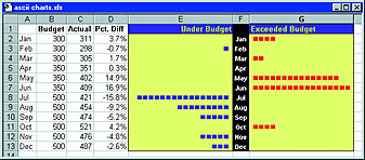 Caption: Formulas in Columns E and G produced this chart by returning a series of Wingdings characters To re-create this chart in Excel, enter the data shown in Columns A through D, and then enter the following formulas: E2: =if(D2<0,rept("n",-round(D2*100,0)),"") F2: =A2 G2: =if(D2>0,rept("n",-round(D2*-100,0)),"") Assign the Wingdings font to cells E2 and G2, and then copy the formulas down the columns to accommodate all the data. Right-align the text in Column E, and adjust any other formatting as you like. Depending on the numerical range of your data, you may need to change the scaling. Experiment by replacing the 100 value in the formulas. You can, of course, substitute any character you like for the n in the formulas to produce a different character in the chart. This technique also works in 1-2-3 and Quattro Pro. Just use the @repeat function in place of Excel's Rept function, and insert an "at" sign (@) before the If and Round functions. û John Walkenbach | Category:spreadsheet Issue: August 1998 |
These Web pages are produced by Australian PC World © 1998 IDG Communications