 Colour Marks the Spot Colour Marks the Spot |
|
Excel's conditional formatting feature (available in Excel 97 or later) offers an easy way to apply special formatting to cells if a particular condition is met. This feature is even more useful when you understand how to use a formula in your conditional formatting specification. FIGURE 2 shows a worksheet with student grades on two tests. Conditional formatting highlights students who scored higher on the second test. This formatting is dynamic; if you change the test scores, the formatting adjusts automatically. 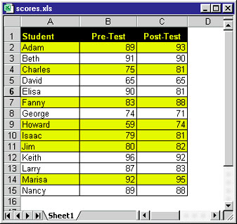 To apply conditional formatting, select range A2:C15 and choose FormatòConditional Formatting. The Conditional Formatting dialog box will appear with two input boxes. In the first box, choose Formula Is, press <Tab>, and enter =$C2>$B2 (meaning, if C2 is greater than B2). Click Format and choose a format to distinguish the cells (I used yellow shading). Click OK, and the formatting will be applied. The conditional formatting formula is evaluated for each cell in the range. The trick here is to use mixed cell references (the column references are absolute, but the row references are relative). To see how this works, activate any cell within the range and choose FormatòConditional Formatting so you can examine the conditional formatting formula for that cell. You'll find that cell A7, for example, uses this formula: =$C7>$B7. |
Category:Spreadsheets Issue: July 2000 |
These Web pages are produced by Australian PC World © 2000 IDG Communications