This page explains the action of the optimisation settings and the information that is reported in the status display after the optimisation phase of rendering has completed.
The settings are:
The reported information (listed below) can be very useful in making subsequent renderings of the same scene go faster.
Some of the terms used above may be unfamiliar to you but in order set the optimisation parameters you will need to understand these terms which arise in the standard ray tracing algorithm and how it is optimised to enable scenes with very large numbers of polygons (faces in the jargon) to be rendered.
The basics of a raytracing algorithm will be explained in this section and then we will move on to consider optimisation techniques. As we do this the nature and use of the raytracing optimisation parameters should become clear. (Hopefully!)
Ray tracing may be a slow procedure but it does give superb photographic quality images. There are many books that describe the theory of ray tracing in detail. A full description of a complete package is given in [1] and there are also many available freeware and shareware ray tracing programs. One of the most comprehensive is POV-Ray which is available from a large number of WWW locations.
The idea on which ray tracing is based seems almost too simple to be true but - here it is:
Follow the paths taken by particles of light (photons) on their journey from light source through the scene (as they are scattered back and forth between objects) and on until they are either captured by the camera or head off to infinity.
In
practice this is a hopeless task because of the huge number of photons emitted
by a light source and the fact that all but a minute fraction of them will ever
be scattered into the camera or eye. So ray tracing does it in reverse. It sends
feelers or rays along the path of the photos from the camera out into the scene.
If the feeler rays find anything they work back towards the sources of illumination
and give us a path for the photons to follow from source to photographic plate.
Sometimes these feeler rays may encounter reflective surfaces and when that
happens they follow a new path and continue their journey. There are lots of
other things that can happen to
feeler rays. Sometimes they may divide with each sub-ray following separate
paths. The way in which the ray tracing algorithm handles such situations
and the sophistication of the mathematical models it uses for light/surface
interaction governs the quality of the images produced.
The standard algorithm for ray tracing can be summarised in five steps:
If when a ray first hits something in the scene it isn't totally absorbed we can continue to trace its path until it reaches a final destination or is so attenuated that there is nothing to see.
So
that's the basic algorithm, but if you have ever experimented with ray tracing
software you probably found that at most you could use about 100 primitive shapes.
Your main observation probably was the hours it took the computer to trace even
an image of moderate resolution. What is worse is that the rendering time increases
as the number of models in the scene increases thus if you need to render a
scene with models made up from thousands of polygons a basic ray tracing renderer
is virtually useless.
So the main question is: Why is ray tracing so much slower? The answer is in
the algorithm, in particular the step: For each pixel test every polygon
and find the one closest to the origin of the ray. This is potentially
an enormous number of operations. For example to synthesize an image of
size 640 by 480 using a 2 by 2 anti-aliasing supersample with a scene of 20,000
polygons requires 24 billion tests.
To try and reduce the time it takes to render a scene with a ray tracer some attempt must be made to try and reduce this enormous number of calculations. A technique we call optimisation.
It is the job of an optimisation routine to divide the scene up in some way so that every ray does not have to be tested against every polygon. Optimisation usually requires two modification to the ray tracing algorithms:
There are two approaches that have received much investigation:
The renderer uses the spatial subdivision method and we will look at that:
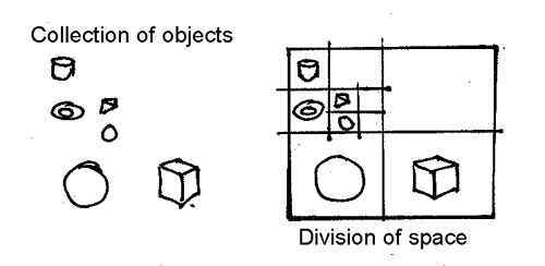
The idea here is to break up space into a number of small boxes so that only a few polygons actually lie in each little box. Then as the rays are traced through the scene we follow them from box to box and check to see if a ray hits any of the polygons lying inside the boxes. If there are only a few polygons in each box we will have considerably reduced the number of calculations and hence the time it takes to render a scene! Ideally putting only one or two polygons in each box (in technical terms the "boxes" are know as "voxels") should be the goal of the first part of the optimisation scheme.
A two dimensional illustration of this principle is given below, it shows a collection of objects and a series of rectangles that divide up the region in which the objects lie so that so that only one object is in each little rectangle:
It is the job of the first optimisation step (scene evaluation) to divide up the scene into the boxes to be used in the later tracing step. There are conflicting goals here, each voxel should have as few polygons (faces) inside them as possible. This implies that they should be small - but if there are too many boxes then the tracing step will not be very fast because as the ray is followed it will have to travel through a very large number of boxes. This is a "balancing act" - technical term "Optimisation". It requires quite a bit of processing to find the best arrangement of the voxels but since many hours of processor time might be saved during rendering it is usually well worth the effort.
One comment worth making: The time it takes to optimise a scene is dependent on the number of polygons in the scene not on the number of pixels in the output picture. So it takes just as long to optimise a scene when rendering a 60 by 40 image as it does for a 1024 by 768 image. However it takes much much longer to trace the image for the larger raster. Thus here again is another very profitable reason to do the best possible job at optimising the scene prior to tracing any rays.
The optimisation step starts by calculating the volume of space occupied by all the faces in the scene to create a bounding box to enclose all the faces in the scene (the so called root node in the octree). If this box contains more than the minimum number of faces it is divided into 8 smaller volumes. These child volumes are checked and any faces assigned to the parent and also fall inside them are put into to a list for each child. If any child box contains more than the minimum number of faces it is further subdivided into 8 sub-volumes, just as its parent's box was. This process is recursive and gives us a tree like structure called an octree, because at each branch there are 8 subdivisions.
This subdivision process for a cubic region of space is illustrated below:
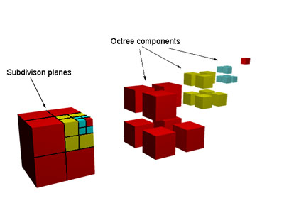
The big cube has been divided into 8, one child node is further divided at each stage. In hierarchical terms the octree resembles:
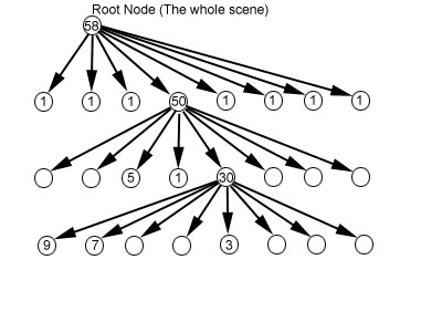
The numbers in the circles represent an example of the number of faces inside the box associated with that node in the octree. You can see that as the subdivision is refined the number of faces in each box decreases. In this particular example the subdivision process is stopped when the number of faces in each box falls below 10.
Once the octree is fully built ray tracing can proceed. Thus when the ray-tracing part of the algorithm follows a ray through the scene it moves from box to box and only a maximum of 10 faces have to tested in each box. A big saving in computation time. The tree structure of the octree makes the task of following a ray through the scene quite quick.
There is a bit of work involved in calculating the movement of the ray and in getting a fairly quick test to see in which box the current position of the traced ray lies but we don't need to worry about this to understand the setting of the ptimisation parameters.
However before actually looking at the parameters there is one complicating issue we must mention:
All this looks great in theory until we come to consider a model made from a connected network of polygonal facets, then we have a bit of a dilemma! A network of connected facets cannot be separated into individual faces. No matter how hard we try, (how may times we subdivide), there is no way that we can separate each polygon so that a rectangle in the subdivision contains only one polygon. The fact that the polygons are connection is responsible for that. The very best we could probably do is associate some polygons with more than one voxel simultaneously. We are going to have to accept that in practice a one polygon to one subdivision goal is unattainable. So we must set a more realistic limit on the number of polygons we are prepared to accept in each voxel.
How close the renderer gets to the 1 to 1 ideal can be determined from the reported information. The (F) value is the number of faces in the scene, the (Fc) value reports how many faces have been placed in voxels. Thus if Fc=F we have a perfect 1 to 1 set-up and the ray tracing should be very fast. The (F/V) value is the maximum number of faces assigned to any one polygon, ideally this should be equal to the desired value (which is set by the Threshold parameter). In most cases we rarely have either Fc=F or F/V = Threshold , any scene in which Fc < 5 F should be regarded as acceptable. In other scenes it is probably worth experimenting with the parameter settings.
[1] Practical Ray Tracing in C / Book and Disk (Wiley Professional Computing) by Craig A. Lindley