The task of rendering three-dimensional graphics primitives is very demanding in terms of memory accesses, integer, and floating-point calculations. There are impressive software rendering packages that handle three dimensional texture-mapped geometry and can generate on the order of 1MPixels/sec on current CPUs. However, the task of rendering graphics primitives is very naturally suited to distribution among separate, specialized pipelined processors. Many of the computations that must be performed are also very repetitive, and so can take advantage of parallelism in a pipeline. This use of special-purpose processors to implement the rendering process is based on some basic assumptions about the requirements of a typical target application. The result can be orders of magnitude increases in rendering performance.
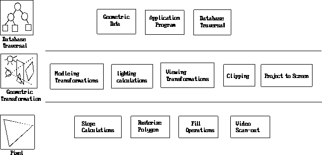
FIGURE 3. The Rendering Pipeline
Each of these stages may be implemented as a separate subsystem. These different stages are all working on different sequential pieces of rendering primitives for the current frame. A more detailed picture of the rendering pipeline is shown in Figure 4. An understanding of the computations that occur at each stage in the rendering process is important for understanding a given implementation and the performance trade-offs made in that implementation. The following is an overview of the basic rendering pipeline, the computational requirements of each stage, and the performance issues that arise in each stage*2[Foley90,Akeley93,Harrell93,Akeley89].
FIGURE 4. The Detailed Stages of the Rendering Pipeline
The CPU Subsystem (Host)
At the top of the graphics pipeline is the main real-time application running on the host. If the host is the limiting stage of the pipeline, the rest of the graphics pipeline will be idle.
The graphics pipeline might really be software running on the host CPU. In which case, the most time consuming operation is likely to be the processing of the millions of pixels that must be rendered. For the rest of this discussion, we assume that there is some dedicated graphics hardware for the graphics subsystem.
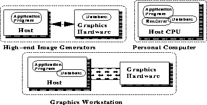
FIGURE 5. Host-Graphics Organizations
The application may itself be multiprocessed and running on one or more CPUs. The host and the graphics pipeline may be tightly connected, sharing a high speed system bus, and possibly even access to host memory. Such buses currently run at several hundred MBytes/sec, up to 1.2GBytes/sec. However, in many high-end visual simulation systems, the host is actually a remote computer that drives the graphics subsystem over a network (SCRAMnet, 100 Mbits/sec, or even ethernet at 10Mbits/sec)

FIGURE 6. Application Traversal Process Pipeline
Possibilities for the application processes are discussed further in Section 6. This section will be focussing on the drawing traversal stage of the application.
Some graphics architectures impose special requirements on the drawing traversal task, such as requiring that the geometry be presented in sorted order from front to back, or requiring that data be presented in large, specially formatted chunks as display lists.
There are three main types of database drawing traversal:
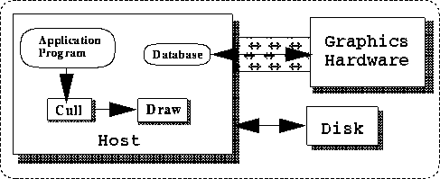
FIGURE 7. Architecture with Shared Database
(5000 tris) * (3 vertices/tri * (8 floats/vertex) * (4bytes/float)) = 480KBytes
--> 28.8 MBytes/sec for a 60fps. update rate.
for just the raw geometric data. The size of geometric data can be reduced through the use of primitives that share vertices, such as triangle strips, or through the use of high-level primitives, such as surfaces, that are expanded in the graphics pipeline (this is discussed further in Section 7). In addition to geometric data, there may also be image data, such as texture maps. It is unlikely that the data for even a single frame will fit a CPU cache so it is important to know the rates that this data can be pulled out of main memory. It is also desirable to not have the CPU be tied up transferring this data, but to have some mechanism whereby the graphics subsystem can pull data directly out of main memory, thereby freeing up the CPU to do other computation. For highly interactive and dynamic applications, it is important to have good performance on transfers of small amounts of data to the graphics subsystems since many small objects may be changing on a per-frame basis.

FIGURE 8. Architecture with Retained Data
The use of retained databases can enable additional processing of the total database by the graphics subsystem. For example, partitioning the database may be done order to implement sophisticated optimization and rendering techniques. One common example is the separation of static from moving objects for the implementation of algorithms requiring sorting. The cost may be additional loss of power and control over the database due to limitations on database construction, such as the number of moving objects allowed in a frame.
The Geometry Subsystem
The second two stages of the rendering pipeline, Figure 3, are commonly called The Geometry Subsystem and The Raster Subsystem, respectively. The geometry subsystem operates on the geometric primitives (surfaces, polygons, lines, points). The actual operations are usually per-vertex operations. The basic set of operations and estimated computational complexity includes [Foley90]: modeling transformation of the vertices and normals from eye-space to world space, per-vertex lighting calculations, viewing projection, clipping, and mapping to screen coordinates. Of these, the lighting calculations are the most costly. A minimal lighting model typically includes emissive, ambient diffuse, and specular illumination for infinite lights and viewer. The basic equation that must be evaluated for each color component (R, G, and B) is [OpenGL93]:
RGBspecular_light*RGBspecular_mat*(half_angle . normal)^shininessMuch of this computation must be re-computed for additional lights. Distance attenuation, local viewing models and local lights add significant computation.
A trivial accept/reject clipping step can be inserted before lighting calculations to save expensive lighting calculations on geometry outside the viewing frustum. However, if an application can do a coarse cull of the database during traversal, a trivial reject test may be more overhead than benefit. Examples of other potential operations that may be computed at this stage include primitive-based antialiasing and occlusion detection.
This block of floating-point operations is an ideal case for both sub-pipelining and block parallelism. For parallelism, knowledge about following issues can help application tuning:
The distribution of primitives to processors can happen in several ways. An obvious scheme is to dole out some fixed number of primitives to processors. This scheme also makes it possible to easily re-combine the data for another distribution scheme for the next major stage in the pipeline. MIMD processors could also receive entire pieces of general display lists, as might be done for parallel traversal of a retained database.
The application can affect the load-balancing of this stage by optimizing the database structure for the distribution mechanism, and controlling changes in the primitive stream.

FIGURE 9. Pixel Operations do many Memory Accesses
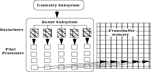
FIGURE 10. Parallelism in the Raster Subsystem
The bottleneck of a pipeline may not be one of the actual stages, but in fact one of the buses connecting two stages, or logic associated with it. There may be logic for parsing the data as it is comes off the bus, or distributing the data among multiple downstream receivers. Any connection that must handle a data explosion, such as the connection between the Geometry and Raster subsystems, is a potential bottleneck. The only way to reduce these bottlenecks is to reduce the amount of raw data that must flow through it, or to send data that requires less processing. The most important connection is the one that connects the graphics pipeline to the host because if that connection is a bottleneck, the entire graphics pipeline will be under-utilized.
The use of FIFO buffers between pipeline stages provides necessary padding that protects a pipeline from the affects of small bottlenecks and smooths the flow of data through the pipeline. Large FIFOs at the front of the pipeline and between each of the major stages can effectively prevent a pipeline from backing up through upstream stages and sitting idle while new data is still waiting at the top to be presented. This is useful important for fill-intensive applications which tend to bottleneck the very last stages in the pipeline. However, once a FIFO fills, the upstream stage will back up.
The final stage in the frame interval is the time spent waiting for the video scan-out to complete for the new frame to be displayed. This period, called a field, is the time from the first pixel on the screen until the last pixel on the screen is scanned out to video. For a 60Hz video refresh rate, the time could be as much as 16.7msecs. Graphics workstations typically use a double-buffered framebuffer so that for an extra field of latency, the system can achieve frame-rates equal to the scan-out rate. A double-buffered system will toggle between two framebuffers, outputting the contents of one framebuffer while the other is receiving rendering results. The framebuffers cannot be swapped until the previous video refresh has completed. This will force the frame rate of the application to run at a integer multiple of the video refresh rate. In the worst case, if the rendering for one frame completed just after a new video refresh was started, the application could theoretically have to wait for the entire refresh period, waiting for an available framebuffer to receive rendering for the next frame.
The time for video refresh is also the lower bound on possible latency for the application. The typical double-buffered application will have a minimum of two fields of latency: one for drawing the next frame while the current one is being scanned, and then a second field for the frame to be scanned. This assumes that the frame rate of the application is equal to the field rate of the video. In reality, a double-buffered application will have a latency that is at least
2 * N * field_timewhere N is the number of fields per application frame.
One obvious way to reduce rendering latency is to reduce the frame time to draw the scene. Another method is to allow certain external inputs, namely viewer position, into later stages of the graphics pipeline. An interesting method to address both of these problems is presented in [Regan94]. A rendering architecture is proposed that handles viewer orientation after rendering to reduce both reduce latency and drawing. The architecture renders a full encapsulating view around the viewer's position. The viewer orientation is sampled after rendering by a separate pipeline that runs at video refresh rate to produce the output RGB stream for video. Additionally, only objects that are moving need to be redrawn as the viewer changes his orientation. Changes in viewer position could also be tolerated by setting a maximum tolerable error in object positions and sizes. Complex objects could even be updated at a slower rate than the application frame rate since their previous renderings still update correctly with viewer orientation.
These principles of sampling viewer position as late as possible, and decoupling of object rendering rate from viewer update rate can also be applied to applications.